
Why Believe in the Gambler's Fallacy?
Although experienced gamblers tend not to believe in the gambler's fallacy, many non-gamblers or novice gamblers do. Today's newsletter provides a partial explanation.
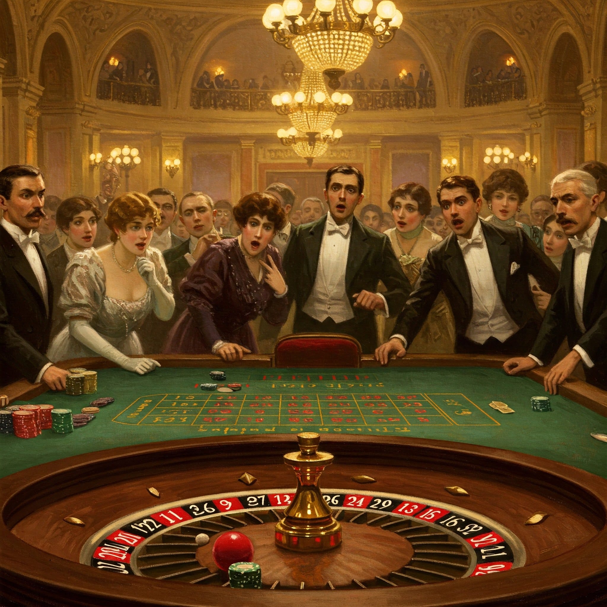
In 1913 in a Monte Carlo casino, a roulette ball landed on black 26 times in a row. With a fair roulette wheel, such a streak—of either color—should occur only once in 68.4 million attempts. Gamblers at that table reportedly lost fortunes betting on red during the course of that improbable streak, incorrectly believing that it must be “due.” The expression of this belief is most often seen among casino gamblers, as with this famous roulette example. As such, along with being called the Monte Carlo fallacy, it is most well-known by the moniker, “the gambler’s fallacy.” The gambler's fallacy is the mistaken belief that chance will self-correct for an improbable series of previous events, even when those events are independent. Gamblers who believe in the fallacy in turn believe that their chances of winning improve by betting against the continuation of the improbable sequence (in this case, by betting on red instead of black).
The gambler’s fallacy has been widely observed and discussed in popular culture and in research on the impact of previous independent events on decision making under risk. I introduced the concept briefly in an earlier post about the Law of Large Numbers noting, however, that most long-term gamblers do not make choices that correspond to belief in the gambler’s fallacy. Nonetheless, many novice gamblers (and non-gamblers) do believe in it. As such, it is worth considering why.
There are three interrelated cognitive “mistakes” associated with belief in the gambler’s fallacy, which I’ll refer to as (1) the representativeness heuristic and insensitivity to sample size; (2) “The Law of Small Numbers” and the belief that chance self-corrects; and (3) overweighting recency. Each will be considered in more detail below.
The Representativeness Heuristic and Insensitivity to Sample Size
Imagine the following scenario:
A certain town is served by two hospitals. In the larger hospital about 45 babies are born each day, and in the smaller hospital about 15 babies are born each day. As you know, about 50% of all babies are boys. However, the exact percentage varies from day to day. Sometimes it may be higher than 50%, sometimes lower.
For a period of 1 year, each hospital recorded the days on which more than 60% of the babies born were boys.
Which hospital do you think recorded more such days?
The larger hospital
The smaller hospital
About the same (that is, within 5% of each other)
Take your time and think about the answer. Scroll down when you’ve decided on the answer.
.
.
.
.
.
.
.
.
.
.
.
.
If you chose Option 3 (about the same), then you will be pleased to know that you answered the same as most participants in a study by the pioneering decision psychologists Amos Tversky and Daniel Kahneman (1974). 22% of their participants chose Option 1 and the same percentage chose Option 2. The other 56% chose Option 3.
Of course, as the discussion of the law of large numbers in the earlier essay suggests, smaller samples are, in fact, more likely to deviate from the population mean than larger samples, and so the correct answer is Option 2. On average, the smaller hospital will have more days with 60% boys than the larger hospital. Indeed, over the course of a year it would be extremely unlikely that the larger hospital would have as many days with more than 60% boys than the larger hospital.
To make this intuitive, imagine flipping a fair coin 10 times. How likely do you think it is that 100% of the outcomes will be heads (keeping in mind that by definition it is a fair coin)? Now imagine the coin has been flipped just three times. Now how likely do you think it is that all outcomes will be heads?
Here the intuition is obvious and correct. Of course, it is more likely that 100% of the outcomes will be heads with just three flips than it is with 10 flips, or, indeed, with any number of flips greater than 3, even though the likelihood of heads for each flip in both cases is 50:50. The math here is pretty simple (if you remember the rule from Probability 101). The chances of n outcomes in a row when the outcome has a probability of p is pn. Thus, the odds of three heads in a row given that there is a 1/2 (50%) likelihood of heads is (1/2)³ (that is 1/8 or 12.5%), meaning that you’ll get all heads one out of each eight attempts, on average over the long run. The chances of ten heads in a row, however, is (1/2)10 (that is 1/1,024), meaning that you would get all heads just 0.10% of the time. You are 128 times more likely to get heads three times in a row than to get heads 10 times in a row. Small samples are more likely to be unrepresentative than large samples.
But in many cases, people are relatively immune to sample size when making likelihood predictions, as the hospital-baby example above demonstrates. In short, people often expect small samples to be more representative of the larger populations from which they are drawn (or—in the case of coin flips and roulette-wheel outcomes—of the probability distribution from which they are drawn). Tversky and Kahneman identify this as an example of what they call the representativeness heuristic, the tendency to assume samples will be representative of the populations from which they are drawn.
Part of the explanation for the gambler’s fallacy no doubt comes from the fact that people believe that an unlikely series of outcomes (say 3 reds in a row) is less normal than it actually is. They expect small samples to be more representative of the populations from which they are drawn than is justified, and so even short streaks are more surprising than they should be. For a live example of this effect with students asked to identify and predict random sequences in coin flips, listen to this section of a Radio Lab podcast, “Stochasticity.”
This is, however, at best a partial explanation for the gambler’s fallacy. It is true that people tend to underestimate the degree to which random, equiprobable outcomes will tend to cluster with small samples (the clustering illusion), as in the roulette and coin flip examples above. As a result, it is also true that people tend to be more surprised by streaks than they ought to be. This does not, however, explain why people would expect subsequent outcomes to be biased in the opposite direction. Indeed, with roulette and other games of chance, a more reasonable application of this incorrect understanding of small samples might be to update one’s beliefs about the game’s outcome likelihoods; that is, to assume that the coin must favor heads or the roulette wheel must be biased to favor black (or whatever color just occurred an unlikely number of times). In that case, people would not believe in the gambler’s fallacy but, on the contrary, they would falsely believe the opposite: that the streak is more likely to continue than chance would predict. After all, if I incorrectly think a coin or a roulette wheel is not behaving randomly, then I might be reasonable to conclude that that device is not random (as discussed here, in the earlier post on law of large number and the importance of experience in evaluating outcome likelihoods). More is needed to explain the gambler’s fallacy.
“The Law of Small Numbers” and the Belief that Chance Self-Corrects
Consider another scenario from Tversky and Kahneman (1971).
The mean IQ of the population of eighth graders in a city is known to be 100. You have selected a random sample of 50 children for a study of educational achievements. The first child tested has an IQ of 150. What do you expect the mean IQ to be for the whole sample?
Take your time and think about the answer before you scroll down to the answer below.
.
.
.
.
.
.
.
.
.
.
.
.
Kahneman and Tversky report that “a surprisingly large number of people believe that the expected IQ of the sample is still 100” (the population mean). The correct answer, they state, is 101.1 The first respondent had an IQ of 150. The other 49 respondents should be expected to have the population average of 100. The mean across all 50 participants would then be 101 [(150+100*49)/50 = 101]. In other words—not only do people expect small samples to be more representative of the larger populations from which they are drawn, as discussed earlier—they also expect chance to somehow self-correct with these small samples, so that the small sample will be representative of the population (or of long-term expectations). They note, as was also noted in the earlier essay about the Law of Large Numbers, that this is not how chance works: “deviations are not canceled as sampling proceeds, they are merely diluted” (p. 106). Yet people often believe that chance will self-correct so that even small samples will maintain the expected outcome ratios that large samples have. They ironically call this false conception of chance, “The Law of Small Numbers.”
It is this combination of both (1) the representativeness heuristic (and the corresponding belief that small samples should look more like the larger samples from which they are drawn), as described in the previous subsection, and (2) the incorrect belief that chance itself will somehow self-correct so that small samples will become representative, that together make up the law of small numbers. And Tversky and Kahneman rightly suggest this helps explain belief in the gambler’s fallacy. As with the representativeness heuristic by itself, however, the belief that chance self-corrects short-term unrepresentative outcomes is still not sufficient.
Overweighting Recency
People could—and often do—falsely believe that chance will self-correct over the long run, while not believing it will do so over the short run. Indeed, this turns out to be a common false belief among experienced gamblers, who instead often believe that chance does not self-correct immediately (that is, over the “short-run”) even while (incorrectly) acknowledging that it does over the long run, in line with their misunderstanding of the law of large numbers. This was referenced earlier and succinctly explained by Kahneman and Tversky with “deviations are not canceled as sampling proceeds, they are merely diluted”; again, see this discussion from the earlier essay on the law of large numbers for an explanation as to why the law of large numbers does not imply that chance must eventually self-correct for an unrepresentative sequence of outcomes). The law of small numbers described above is not just dependent on the false belief that chance will eventually self-correct, but rather that chance will self-correct over the short-term.
This belief relies on an overweighting of recent events. If people who believe in the gambler’s fallacy see a streak of red outcomes in roulette, they do not tend to consider the ratio of reds to blacks over the previous hundred (or thousand, or even just 10) outcomes. Instead, they tend to focus on the most recent streak, even if it is just a few reds in a row. If they were paying attention to a longer series of previous outcomes, they might correctly conclude that even three reds in a row would not be enough to balance out the ratio of reds to blacks, and conclude that more reds are still “due,” while continuing to believe in the gambler’s fallacy. Of course, gamblers might do that, and some gamblers would do that. In my opinion, it would be fair to call that an example of the gambler’s fallacy, since the fallacy itself is not consistently defined except to point to a false and unjustified belief that chance will self-correct. That said, most people who demonstrate belief in the gambler’s fallacy overweight the importance of recent events, as would be suggested by Tversky and Kahneman’s tongue-in-cheek “Law of Small Numbers.”
In summary, belief in the gambler’s fallacy usually corresponds to holding this trifecta of unjustified beliefs: (1) the expectation that small samples will be more representative of long-term likelihood distributions they tend to be; (2) the belief that chance must self-correct so that short-term unrepresentative distributions will not violate long-term expectations; and (3) the overweighting of recent outcomes, even when longer sequences of outcomes are available to memory and could be taken into account.
If you feel uneasy about the explanation so far, you should. The current explanation points to three false beliefs that together describe the gambler’s fallacy, but it does not explain why people have those false beliefs. Kahneman and Tversky’s representativness heuristic partly explains it, since that heuristic is justifiably posited to be generally adaptive even if it misfires in certain contexts, such as at the roulette table. But, again, the representativeness heuristic is not enough to explain why people would think chance self-corrects or why they pay more attention to immediately preceding outcomes than to longer sequences of events. The upcoming essays will address some of these concerns.
They consider how widespread belief in the gambler’s fallacy is, discussing examples from casino blackjack, roulette, and slot machines. Ultimately, these essays will argue that despite a variety of reasons to believe that the gambler’s fallacy is a widespread phenomenon in games of chance, the attrribution of the fallacy to gambler’s is largely itself a fallacy, resulting from a wide variety of mistaken assumptions or attributions.
The insertion of “they state” is to note that their math deserves to be challenged, and for at least two reasons. First, they state that the IQ of a population of 8th graders in a city is known to be 100. But they do not state that their sample is drawn from that population. They only state that they have selected a random sample of children. One plausible interpretation of the first child with an IQ of 150 is that it suggests some increased likelihood that the child is not an 8th grader or not from that city, and that populations of children may have higher IQs (as is in fact the case for some populations, and perhaps for a random sample of children across the population of all children).
Second, even if participants assume—as Tversky and Kahneman intended—that the sample is drawn from the aforementioned population of 8th graders in a particular city, their math assumes that that population is so large as to be irrelevant. Of course, if the population of 8th graders in a city is 1 million, then they would be correct to conclude that the first student with an IQ of 150 has no meaningful impact on the mean IQ of the rest of the sample. But if the city only has 50 eighth graders, then respondents believing the mean IQ should be 100 would be correct, and the IQ of the other 49 participants should be something less than 100, “correcting for chance.” This is because events are not independent given a known non-infinite population mean: the sample was taken from the population and so any participants that are non-representative will impact correct estimates of the remaining members of the population, in the opposite direction. Given a known distribution of a limited population, likelihoods do self-correct because events are not independent. They are negatively dependent.
There is one reason why this is just a footnote rather than being in the main text, and there are two reasons for not leaving this footnote out altogether. It’s just a footnote because it turns out that Tversky and Kahneman are nonetheless correct, and they get their evidence from a variety of other sources as well. It’s also somewhat reasonable for them to claim the right answer is 101, since most cities will have a population of 8th graders in the thousands, and so the impact would still round to 101 (although it would nonetheless be something less than 101 before rounding, since that student with 150 was removed from that population and will impact the mean score of the remaining members of the population). Tversky and Kahneman are correct that many people do believe that chance itself will self-correct over the short term, even for independent events like coin flips or the outcomes of a roulette wheel spin. As such, pointing to problems with this scenario are a bit of a red herring.
The two reason for leaving it in as a footnote, however, are, first, because it points to a central theme from the earlier essay about the law of large numbers: in the wild, it is rarely the case that events are independent and that previous outcomes are irrelevant to subsequent outcome likelihoods. The heuristic of assuming chance will self-correct turns out to be accurate given a known and limited population (as is the case in their scenario).
Second, it points to a common concern with scenarios devised to demonstrate cognitive heuristics and biases more generally. The scenarios are often subject to similar criticisms, designed so as to get the maximum effect size, and as a result implying participants are less rational than in fact they might be. To the extent that outcomes are rarely independent in the wild, participants could be adaptive to update their probabilities based on an initial sample (in this case, a sample of one with an IQ of 150), even if it would be a mistake in the hypothetical scenario they are given in an experiment. Furthermore, if they correctly interpret the sample as coming from that population of 8th graders in the city of unknown size, they would be right to assume that the rest of the sample should correct to some degree for the unrepresentative first child. In this case, it was Tversky & Kahneman who missed recognizing that with a known population mean and a limited population, any sample from that population will change the likelihoods of subsequent samples from that population and that chance will “self-correct” (however small that self-correction might be, which cannot be determined without knowing the population size of those hypothetical 8th graders in that hypothetical city).